Draw fitted and implied models with ggplot2

geom_model() adds a model to an ordinary ggplot2::ggplot(). A supplied model may be a fit from stats::lm() or stats::aov(), or a two-sided formula that is fitted once against the layer data. With no model, the layer draws the model implied by its mapped positions, separately in each panel and group.

Usage

geom_model(
  mapping = NULL,
  data = NULL,
  stat = "model",
  position = "identity",
  ...,
  model = NULL,
  orientation = NA,
  na.rm = FALSE,
  show.legend = NA,
  inherit.aes = TRUE
)

stat_model(
  mapping = NULL,
  data = NULL,
  geom = "model",
  position = "identity",
  ...,
  model = NULL,
  orientation = NA,
  na.rm = FALSE,
  show.legend = NA,
  inherit.aes = TRUE
)

Arguments

mapping, data, position, show.legend, inherit.aes

See ggplot2::geom_smooth(). data may be a data frame, a function, or a one-sided formula.

stat

The statistical transformation. Defaults to "model".

...

Fixed aesthetics and other layer parameters. For an inferred continuous model these include formula, se, n, fullrange, level, and method.args, with the meanings used by ggplot2::stat_smooth(). width controls categorical model marks. With a supplied model, n controls the prediction grid. se = TRUE requires an inferred continuous model; it is refused when model is supplied.

model

A fitted lm or aov, a two-sided model formula, or NULL to draw the model implied by the mapped positions.

orientation

Layer orientation. "x" puts the outcome on y; "y" puts it on x. NA uses the mapped model outcome for a supplied model, and ggplot2's orientation rules for an inferred model.

na.rm

If FALSE, missing values are removed with a warning. If TRUE, they are removed silently.

geom

The geometric object. stat_model() defaults to "model".

Value

A ggplot2 layer.

Details

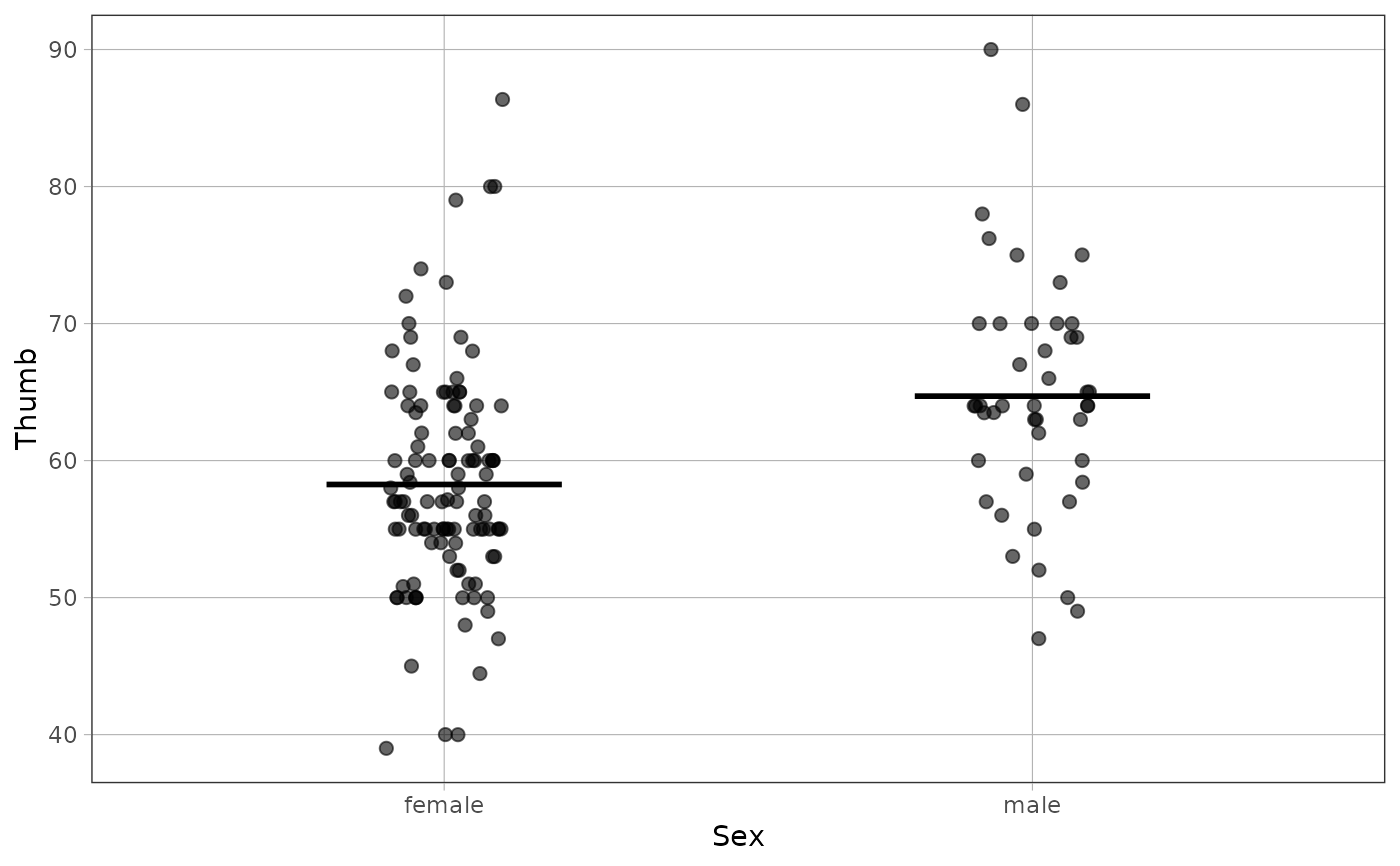
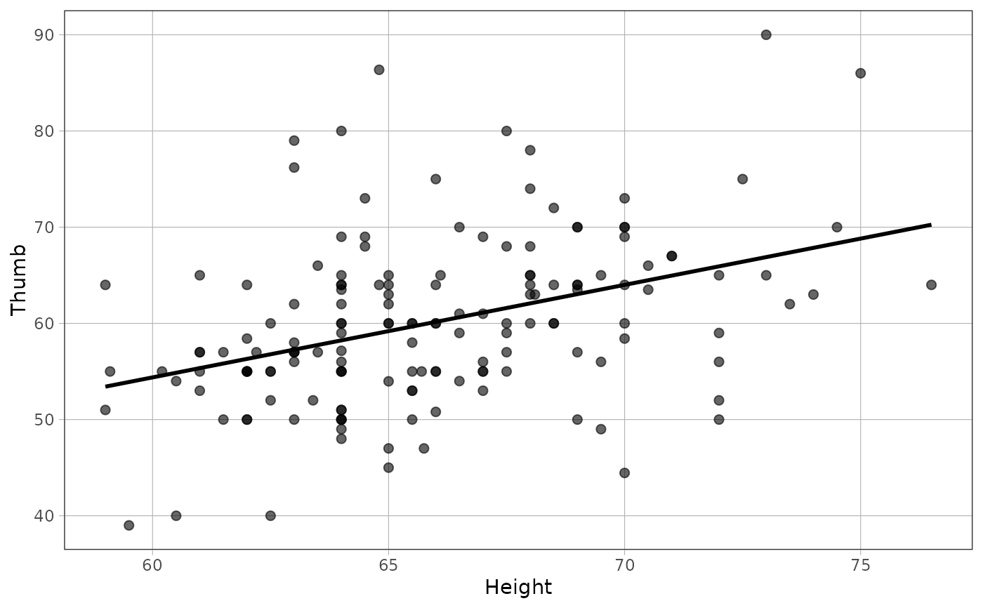
Empty models draw an intercept, numeric predictors draw fitted lines, and categorical predictors draw one short mark per group. A model with one numeric and one categorical predictor draws one line per category.

A supplied model is one fixed claim evaluated on a prediction grid built from the layer data.

The displayed predictor is read from the plot mapping or this layer's local mapping. One additional predictor may be present in the data: categories produce separate traces, and numeric values use the mean and mean plus or minus one standard deviation. Outcome-axis expressions such as log(y) are applied to the predictions. A supplied model is prepared once when added to the plot, including when data is a function or formula.

Override unrelated inherited aesthetics locally, or set inherit.aes = FALSE and supply a predictor mapping such as aes(x = Height). Without explicit data or positions, the layer follows the first observation layer, preferring points, so a model describes the rows and axes the plot actually shows.

Examples

fit <- lm(Thumb ~ Height, data = Fingers)
ggplot2::ggplot(Fingers, ggplot2::aes(Height, Thumb)) +
  ggplot2::geom_point() +
  geom_model(model = fit)


group_fit <- lm(Thumb ~ Sex, data = Fingers)
ggplot2::ggplot(Fingers, ggplot2::aes(Sex, Thumb)) +
  ggplot2::geom_jitter(width = 0.1) +
  geom_model(model = group_fit)