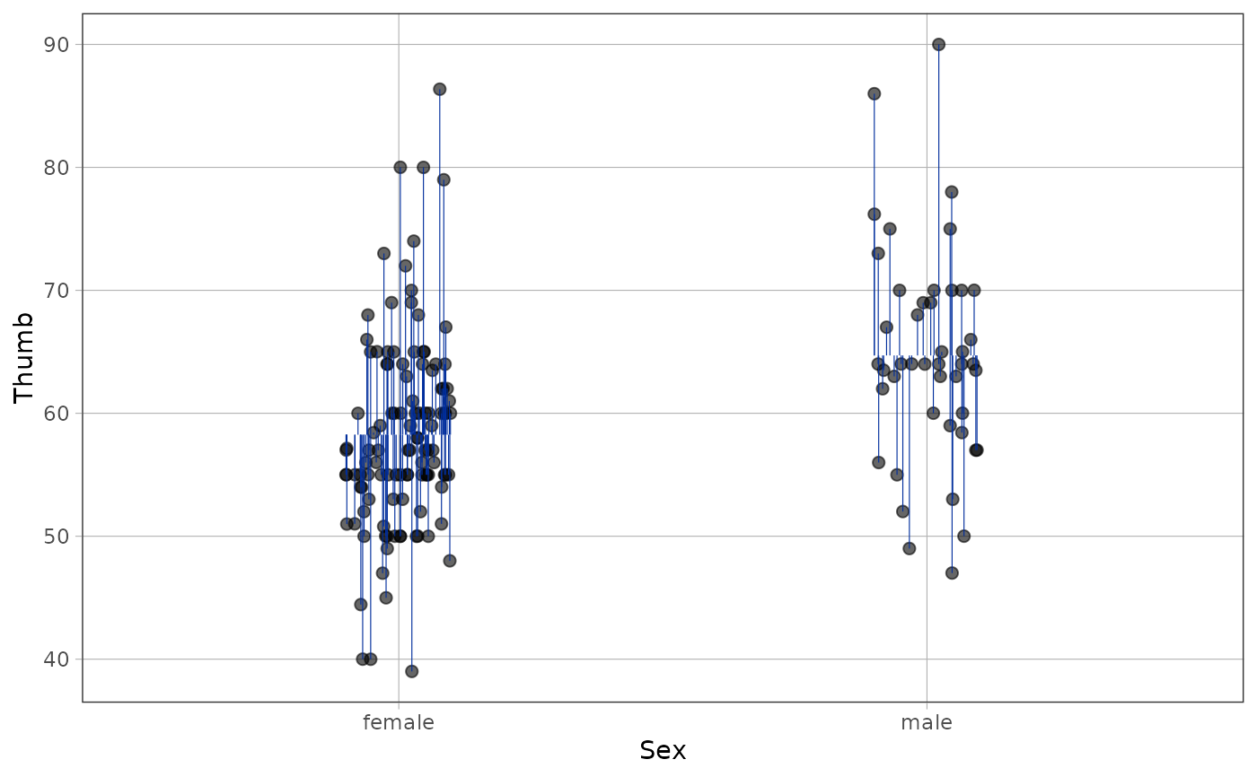
Residual and reduction layers for ggplot2 — geom

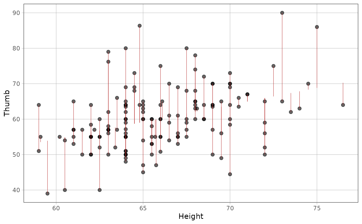
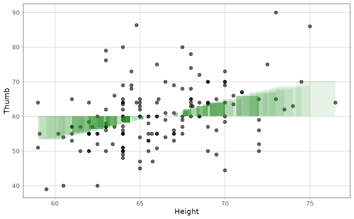
These layers measure a fitted model directly from an ordinary ggplot2::ggplot(). A residual segment runs from the model's prediction to the observed value; an arrow at its last end points to the observation. A reduction segment runs from the prediction to the model's grand mean. The square variants draw areas proportional to those squared distances at a shared aspect ratio.

Usage

geom_resid(
  mapping = NULL,
  data = NULL,
  stat = "resid",
  position = "identity",
  ...,
  model = NULL,
  fun = NULL,
  orientation = NA,
  linewidth = 0.2,
  na.rm = FALSE,
  show.legend = NA,
  inherit.aes = TRUE
)

geom_square_resid(
  mapping = NULL,
  data = NULL,
  stat = "resid",
  position = "identity",
  ...,
  model = NULL,
  fun = NULL,
  orientation = NA,
  aspect = 4/6,
  alpha = 0.1,
  na.rm = FALSE,
  show.legend = NA,
  inherit.aes = TRUE
)

geom_reduce(
  mapping = NULL,
  data = NULL,
  stat = "reduce",
  position = "identity",
  ...,
  model = NULL,
  fun = NULL,
  orientation = NA,
  linewidth = 0.2,
  na.rm = FALSE,
  show.legend = NA,
  inherit.aes = TRUE
)

geom_square_reduce(
  mapping = NULL,
  data = NULL,
  stat = "reduce",
  position = "identity",
  ...,
  model = NULL,
  fun = NULL,
  orientation = NA,
  aspect = 4/6,
  alpha = 0.1,
  na.rm = FALSE,
  show.legend = NA,
  inherit.aes = TRUE
)

stat_resid(
  mapping = NULL,
  data = NULL,
  geom = "resid",
  position = "identity",
  ...,
  model = NULL,
  fun = NULL,
  orientation = NA,
  na.rm = FALSE,
  show.legend = NA,
  inherit.aes = TRUE
)

stat_reduce(
  mapping = NULL,
  data = NULL,
  geom = "resid",
  position = "identity",
  ...,
  model = NULL,
  fun = NULL,
  orientation = NA,
  na.rm = FALSE,
  show.legend = NA,
  inherit.aes = TRUE
)

Arguments

mapping, data, position, show.legend, inherit.aes: See ggplot2::geom_segment(). data may also be a function or one-sided formula; predictions are added after that function has selected its rows.
stat: The statistical transformation to use. The geom constructors use "resid" or "reduce" by default.
...: Other arguments passed to ggplot2::layer(). These are usually fixed aesthetics such as colour, fill, alpha, or linetype.
model: A model already fit by stats::lm() or stats::aov(). Name this argument in a ggplot2 call, as in geom_resid(model = fit).
fun: For residual layers, a function instead of model. It receives the mapped predictor values and returns predicted outcomes. The default orientation predicts y from x; orientation = "y" predicts x from y. Supply only one of model and fun. Reductions require a fitted model.
orientation: Layer orientation. NA infers a model's outcome axis; "x" puts it on y and "y" puts it on x. For fun, NA means "x".
linewidth: The line width. The default is 0.2.
na.rm: If FALSE, the default, missing observations are removed with a warning. If TRUE, they are removed silently.
aspect: The square's aspect ratio. The default is 4 / 6.
alpha: The square's transparency. The default is 0.1.
geom: The geometric object to use. The stat constructors use "resid" by default; use "square_resid" to draw areas.

Value

A ggplot2 layer.

Details

When the observations have their own data or mappings, these layers follow the first point layer (or the first non-annotation layer when there are no points). Explicit layer data and mapping arguments take precedence.

With orientation = NA, a model's outcome determines the direction. The outcome expression must match an axis exactly: log(y) is refused for a model of y, because that distance is not the model's residual. An explicit orientation = "x" puts the outcome on y; "y" puts it on x and must agree with that mapping. Coordinate systems such as ggplot2::coord_flip() are applied later and do not change this argument.

A jittered point layer and its model layer must use the same ggplot2::position_jitter() object with a numeric seed. The model layer keeps the fitted endpoint fixed while moving the observed endpoint by the same amount as its point.

Positional expressions are evaluated reproducibly on the current data, so random mappings give the observations and residuals the same coordinates. Native layers still respond to later data and mapping changes. A new unseeded random mapping must be added before the residual layer, or carry its own fixed seed. Checks that need the rows or mappings run when the plot is built: axes, prediction, outcome axis, then reduction eligibility.

Native square layers inherit mapped aesthetics by default, including colour. gf_square_resid() and gf_square_reduce() default to inherit = FALSE for neutral square outlines. Set their inherit = TRUE to match this API.

Reduction layers express the ordinary least-squares sum-of-squares identity. They require an unweighted model with an intercept, no offset, and its stored model frame. On the fitted observations, the identity holds across the sums of the square areas, not separately for each observation or for new prediction data.

Examples

model <- lm(Thumb ~ Height, data = Fingers)
ggplot2::ggplot(Fingers, ggplot2::aes(Height, Thumb)) +
  ggplot2::geom_point() +
  geom_resid(model = model, colour = "firebrick")


ggplot2::ggplot(Fingers, ggplot2::aes(Height, Thumb)) +
  ggplot2::geom_point() +
  geom_square_reduce(model = model, fill = "forestgreen")


jitter <- ggplot2::position_jitter(width = 0.1, seed = 42)
group_model <- lm(Thumb ~ Sex, data = Fingers)
ggplot2::ggplot(Fingers, ggplot2::aes(Sex, Thumb)) +
  ggplot2::geom_point(position = jitter) +
  geom_resid(model = group_model, position = jitter)