Find a percentage of a distribution

Given a distribution, find which values lie in the upper, lower, or middle proportion of the distribution. Useful when you want to do something like shade in the middle 95% of a plot. This is a greedy operation, meaning that if the cutoff point is between two whole numbers the specified region will suck up the extra space. For example, the requesting the upper 30% of the [1 2 3 4] will return [FALSE FALSE TRUE TRUE] because the 30% was greedy.

outer() marks values in both outer tails of a distribution. It is the complement of middle(): outer(x, prop) is equivalent to tails(x, 1 - prop).

Usage

middle(x, prop = 0.95, greedy = TRUE)

outer(x, prop)

tails(x, prop = 0.95, greedy = TRUE)

lower(x, prop = 0.025, greedy = TRUE)

upper(x, prop = 0.025, greedy = TRUE)

Arguments

x

The distribution of values to check.

prop

The total proportion in both tails combined, must be in (0, 1).

greedy

Whether the function should be greedy, as per the description above.

Value

A logical vector indicating which values are in the specified region.

Details

Note that NA values are ignored, i.e. they will always return FALSE.

See also

The sampling distributions guide walks through building these distributions with do() and shuffle(), and shows the bootstrap variant: https://coursekata.github.io/coursekata-r/articles/sampling-distributions.html

Examples

# each function returns a logical vector marking the values in its region
upper(1:10, .1)
#>  [1] FALSE FALSE FALSE FALSE FALSE FALSE FALSE FALSE FALSE  TRUE
lower(1:10, .2)
#>  [1]  TRUE  TRUE FALSE FALSE FALSE FALSE FALSE FALSE FALSE FALSE
middle(1:10, .5)
#>  [1] FALSE FALSE  TRUE  TRUE  TRUE  TRUE  TRUE  TRUE FALSE FALSE
tails(1:10, .5)
#>  [1]  TRUE  TRUE FALSE FALSE FALSE FALSE FALSE FALSE  TRUE  TRUE

# they are most often used as the fill aesthetic of a histogram of a
# sampling distribution -- here, b1s estimated from shuffled (null) data
set.seed(42)
shuffled <- data.frame(b1 = replicate(200, {
  shuffled_tip <- base::sample(TipExperiment$Tip)
  b1(lm(shuffled_tip ~ Condition, data = TipExperiment))
}))

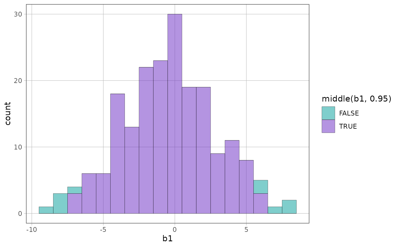
# color the middle 95%: the b1 values we would expect to see often
# if the empty model were true
gf_histogram(~b1, data = shuffled, binwidth = 1, fill = ~ middle(b1, .95))


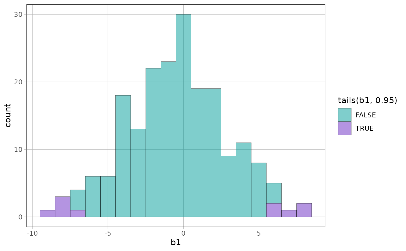
# tails() marks the same cutoffs with the opposite coloring: the values
# outside the middle 95% are the 5% most extreme
gf_histogram(~b1, data = shuffled, binwidth = 1, fill = ~ tails(b1, .95))


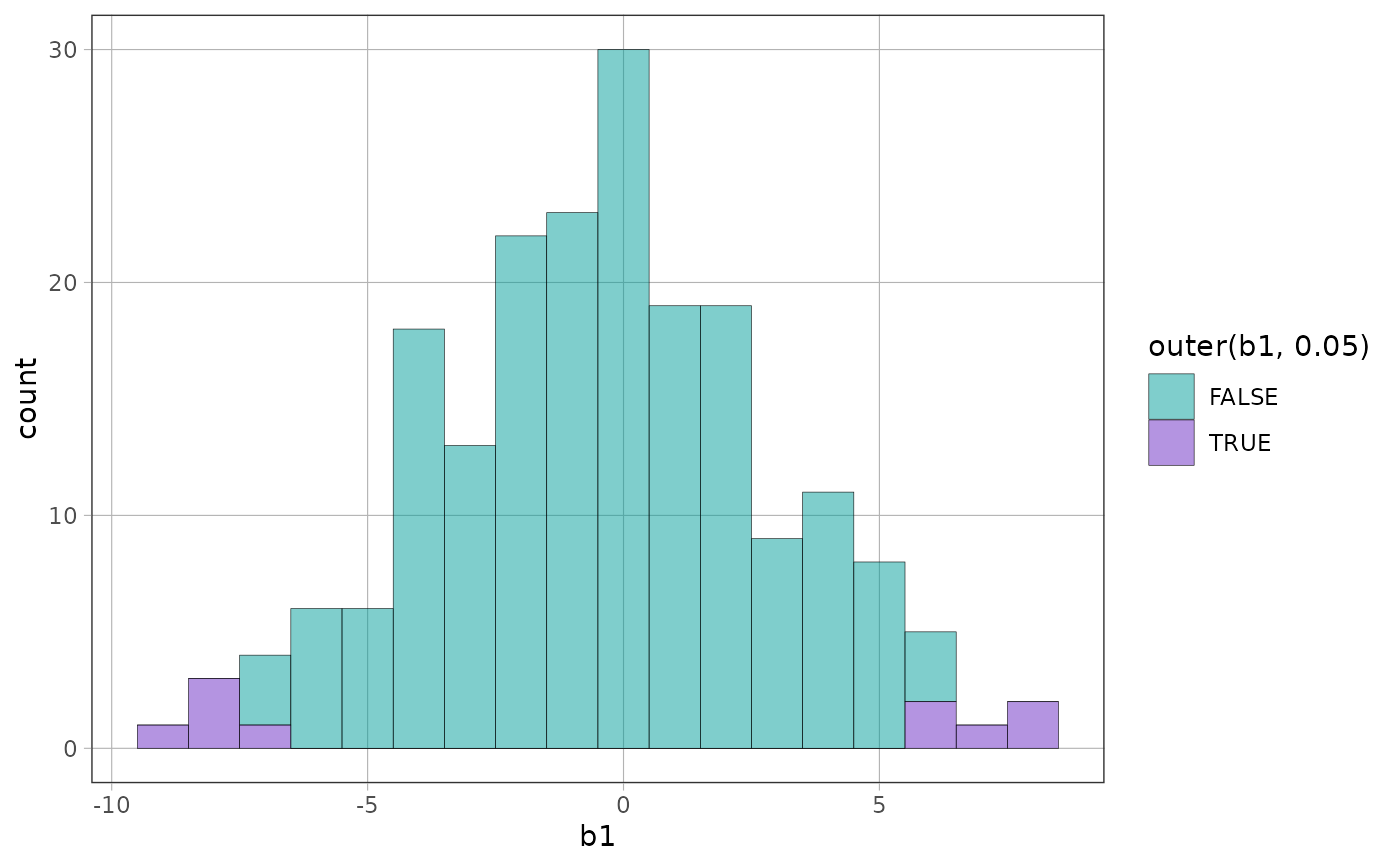
# outer() marks the same region as tails() but takes the tail proportion
# directly: the outer 5%
gf_histogram(~b1, data = shuffled, binwidth = 1, fill = ~ outer(b1, .05))


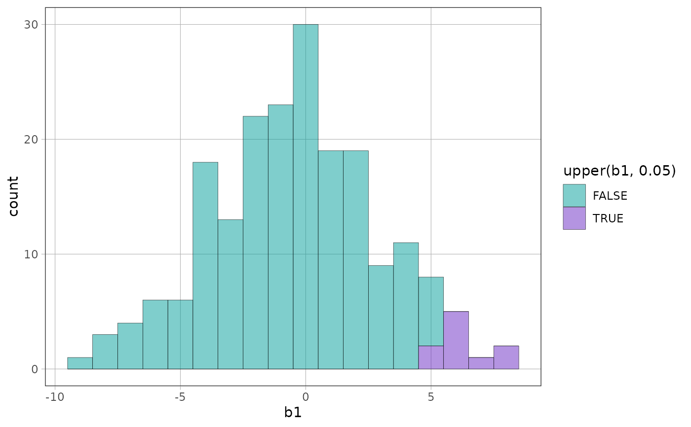
# upper() and lower() are for directional hypotheses: all 5% goes in one tail
gf_histogram(~b1, data = shuffled, binwidth = 1, fill = ~ upper(b1, .05))

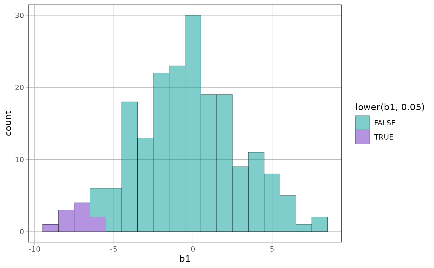
gf_histogram(~b1, data = shuffled, binwidth = 1, fill = ~ lower(b1, .05))