Add Reduction Lines to a Plot — gf

Draws reduction lines from the value a fitted model predicts for each observation to the grand mean. Squaring and summing those lengths across observations gives the model sum of squares; gf_resid() supplies the error term in the same decomposition. Each line runs along whichever axis the plot puts the model's outcome on, so a model of the variable drawn on x is measured across x rather than down y.

Usage

gf_reduce(
  object = NULL,
  gformula = NULL,
  data = NULL,
  ...,
  model,
  linewidth = 0.2,
  xlab,
  ylab,
  title,
  subtitle,
  caption,
  geom = coursekata::GeomResid,
  stat = coursekata::StatReduce,
  position = "identity",
  show.legend = NA,
  show.help = NULL,
  inherit = TRUE,
  environment = parent.frame()
)

Arguments

object: A ggformula plot object, typically created with gf_point().
gformula: Not used. gf_reduce() measures a model, not an aesthetic formula; a model given positionally lands here and is moved to model.
data: Not used. The reductions are measured over the data the plot was built from. Anything supplied here is left for ggformula and ggplot2 to answer, exactly as it is for any other gf_ layer.
...: Additional arguments. Typically these are (a) ggplot2 aesthetics to be set with attribute = value, such as color, alpha or linetype, (b) ggplot2 aesthetics to be mapped with attribute = ~ expression, or (c) attributes of the layer as a whole.
model: A model already fit by lm() or aov(). The plot supplies the observations' position on the other axis; the model supplies what it predicted for each of them. May be given positionally or as model =. A fit without an intercept, or one fit with weights or an offset, is refused. For an unweighted least-squares fit with an intercept, the sum of squared total deviations equals the sum of squared residuals plus the sum of squared reductions. That identity need not hold without an intercept. Weighted least squares instead guarantees a weighted identity based on a weighted mean, which the plot's plain areas do not represent. gf_resid() can measure either fit because it does not rely on the decomposition.
linewidth: The width of the reduction lines. Default is 0.2. Must be named.
xlab, ylab, title, subtitle, caption: Labels for the plot.
geom, stat, position: Not set by the caller. A reduction is drawn by its own geom and stat, with a jitter that holds the outcome axis still so its segments start at the grand mean without floating off it, while jittering the other axis exactly the points layer's own jitter did.
show.legend: Whether this layer contributes to the legend.
show.help: Print the layer's own help instead of drawing.
inherit: Whether the layer inherits the plot's aesthetics. The axes and the prediction are stated outright; everything else – a mapped color, for instance – is inherited from the plot.
environment: The environment mappings are resolved in.

Value

A ggplot object with reduction lines added.

Details

The grand mean is the model's own, mean() of the outcome column the model was fit on, not anything read off the plot's data. On a faceted plot that is one number for every panel: every panel is measured against the same line, which is what makes the picture in each panel a piece of one decomposition rather than a decomposition of its own.

Examples

set.seed(1)
penguins_20 <- sample(penguins, 20)

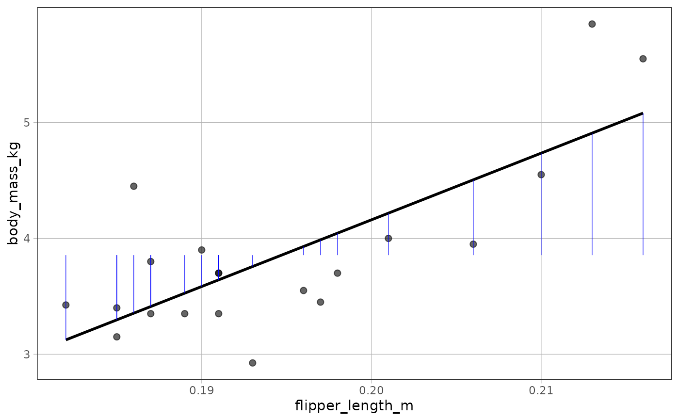
# the reduction: how far a model's fit moves the prediction from the grand
# mean, for a regression model
flipper_model <- lm(body_mass_kg ~ flipper_length_m, data = penguins_20)
gf_point(body_mass_kg ~ flipper_length_m, data = penguins_20) %>%
  gf_model(flipper_model) %>%
  gf_reduce(flipper_model, color = "blue")


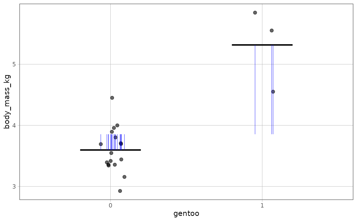
# and for a two-group model on a jitter plot
gentoo_model <- lm(body_mass_kg ~ gentoo, data = penguins_20)
gf_jitter(body_mass_kg ~ gentoo, data = penguins_20, width = .1) %>%
  gf_model(gentoo_model) %>%
  gf_reduce(gentoo_model, color = "blue")


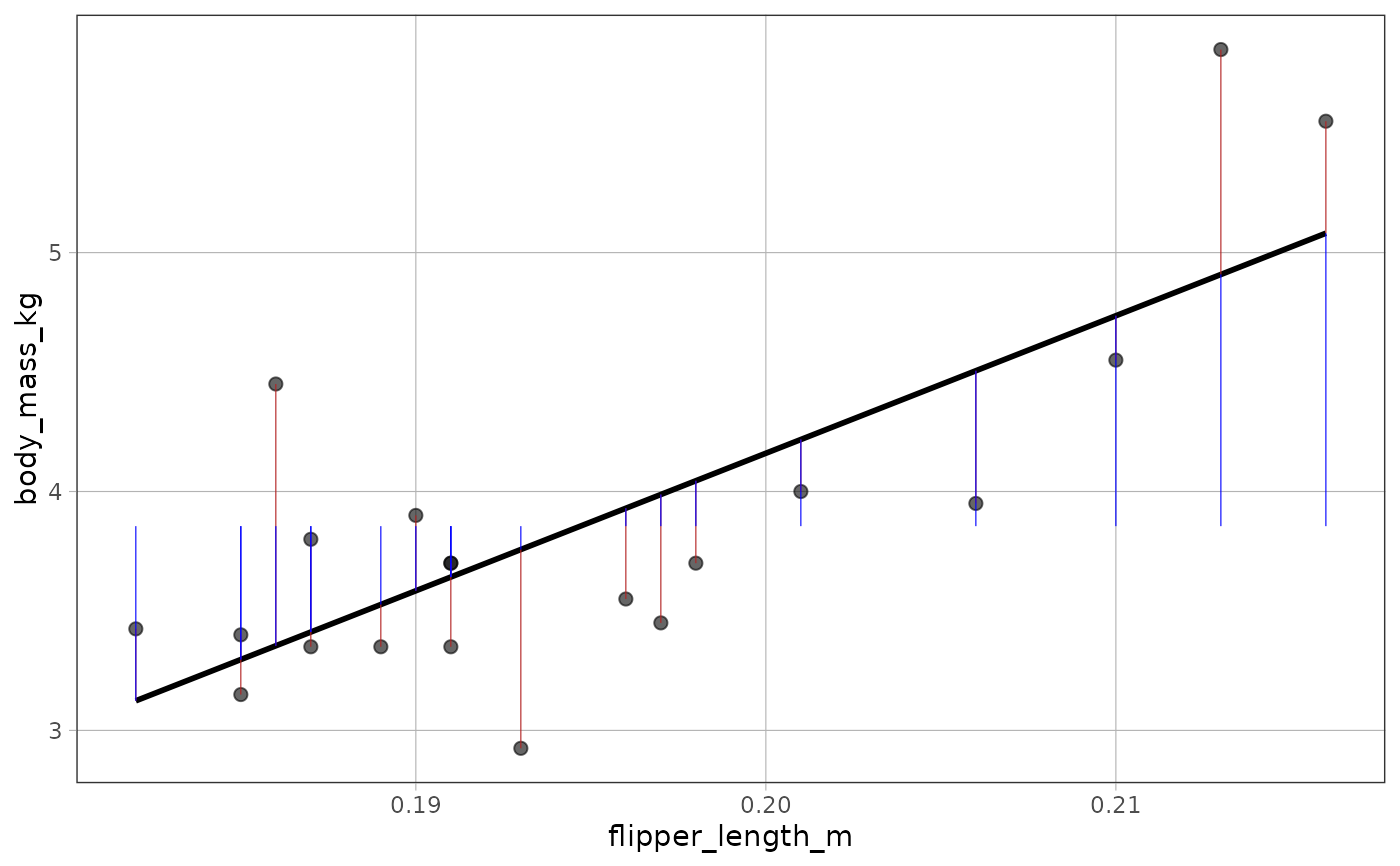
# each observation's signed deviation from the grand mean is its residual
# (firebrick) plus its reduction (blue)
gf_point(body_mass_kg ~ flipper_length_m, data = penguins_20) %>%
  gf_model(flipper_model) %>%
  gf_resid(flipper_model, color = "firebrick") %>%
  gf_reduce(flipper_model, color = "blue")