Annotate a model's coefficients on a plot

Draws the intercept and slope (or group differences) of a fitted model as arrows and labels directly on the plot they describe: a rise-over-run triangle for a continuous predictor, an arrow to each non-reference group for a categorical one. Where gf_model() draws the fit itself, gf_b() draws the numbers that describe it.

gf_coef() is a fully supported alias of gf_b(). The package already exports b(), b0(), b1() as its vocabulary for coefficients, and a reader who knows stats::coef() will look for a plot-side counterpart under that name.

Usage

gf_b(
  object = NULL,
  gformula = NULL,
  data = NULL,
  ...,
  model,
  color = "#b599ed",
  label_color = "black",
  label_size = 3.5,
  arrow_linewidth = 0.5,
  show_b0 = TRUE,
  run = NULL,
  run_x = NULL,
  b0_alpha = 0.3,
  b0_linewidth = 0.8,
  b0_size = 4,
  arrow_nudge = 0.18,
  label_nudge = 0.08,
  xlab,
  ylab,
  title,
  subtitle,
  caption,
  geom = ggplot2::GeomSegment,
  stat = "identity",
  position = "identity",
  show.legend = NA,
  show.help = NULL,
  inherit = TRUE,
  environment = parent.frame()
)

gf_coef(
  object = NULL,
  gformula = NULL,
  data = NULL,
  ...,
  model,
  color = "#b599ed",
  label_color = "black",
  label_size = 3.5,
  arrow_linewidth = 0.5,
  show_b0 = TRUE,
  run = NULL,
  run_x = NULL,
  b0_alpha = 0.3,
  b0_linewidth = 0.8,
  b0_size = 4,
  arrow_nudge = 0.18,
  label_nudge = 0.08,
  xlab,
  ylab,
  title,
  subtitle,
  caption,
  geom = ggplot2::GeomSegment,
  stat = "identity",
  position = "identity",
  show.legend = NA,
  show.help = NULL,
  inherit = TRUE,
  environment = parent.frame()
)

Arguments

object: A plot created with the ggformula package.
gformula: Not used. gf_b() annotates a model, not an aesthetic formula; a model given positionally lands here and is moved to model.
data: Not used. The marks are placed from the model's own coefficients and data.
...: Not used. Every mark states its own geom and params; set appearance with color, label_color, label_size, arrow_linewidth, b0_linewidth, b0_size, b0_alpha. Anything else here (alpha, linetype, ...) is warned about and dropped, because the marks are heterogeneous geoms with no single params bag to receive it.
model: The model to annotate: a fit from lm() or aov(), with one predictor at most, and that predictor spelled the way the plot's own axis spells it – log(Height) and Height are the same column but not the same axis, and b1 is a rise per unit of whichever one the model was fit on. It needs an intercept, because every mark here is measured from b0; a categorical predictor needs treatment coding, because every arrow is drawn as one group's difference from the reference group and no other coding's coefficients are that. Each of those is refused rather than drawn, because each would otherwise produce a picture that looks right. A formula is refused too – gf_b()'s whole output is a set of labeled numbers, and there is no fit to read them from. May be given positionally or as model =. Omitted, the model the plot implies is fit and annotated instead.
color, label_color: The arrows/lines and the label text. colour and label_colour are accepted too. Each is a single value, not a mapping – every mark is one row computed from the coefficients, so there are no rows of data to map an aesthetic over; color = ~variable is refused.
label_size, arrow_linewidth, b0_linewidth, b0_size: Sizes for the labels, the arrows, the b0 line and the b0 dot.
show_b0: Draw the b0 line/dot and its label, and expand the PREDICTOR's axis to include 0 on a continuous model – x on most plots, y on one that puts the outcome on x. TRUE by default; a later gf_lims() on that axis overrides the expansion and can push the b0 dot off the page.
run, run_x: The run a continuous model's rise is measured over, and the x position the triangle starts at. Both chosen from the data when left NULL. Naming run on a categorical model is warned about and ignored – its coefficients are group differences, not a rate.
b0_alpha: The transparency of the categorical b0 reference line.
arrow_nudge, label_nudge: A categorical arrow's x position, and its label's offset from it, in level units (1 = one group apart). Not used on the empty model, whose one axis is a count, not a level, and whose b0 label is placed at the panel's edge instead.
xlab, ylab, title, subtitle, caption: Labels for the plot.
geom, stat, position: Not set by the caller. Every mark states its own geom.
show.legend: Not used. The marks are annotations and never contribute to a legend; a non-default value is warned about and dropped.
show.help: Print the function's own help instead of drawing.
inherit: Not set by the caller. Every mark states its own aesthetics.
environment: The environment mappings are resolved in.

Value

A ggplot object with the model's coefficients annotated on it.

What is drawn

A continuous predictor: a vertical rise arrow from fit(run_x) to fit(run_x + run), a horizontal run segment at its tip, a rise label (plotmath b1 when run is 1, otherwise run times b1), a run-distance label under the run segment (over it, for a negative rise), and a hollow dot at (0, b0) with a b0 label.

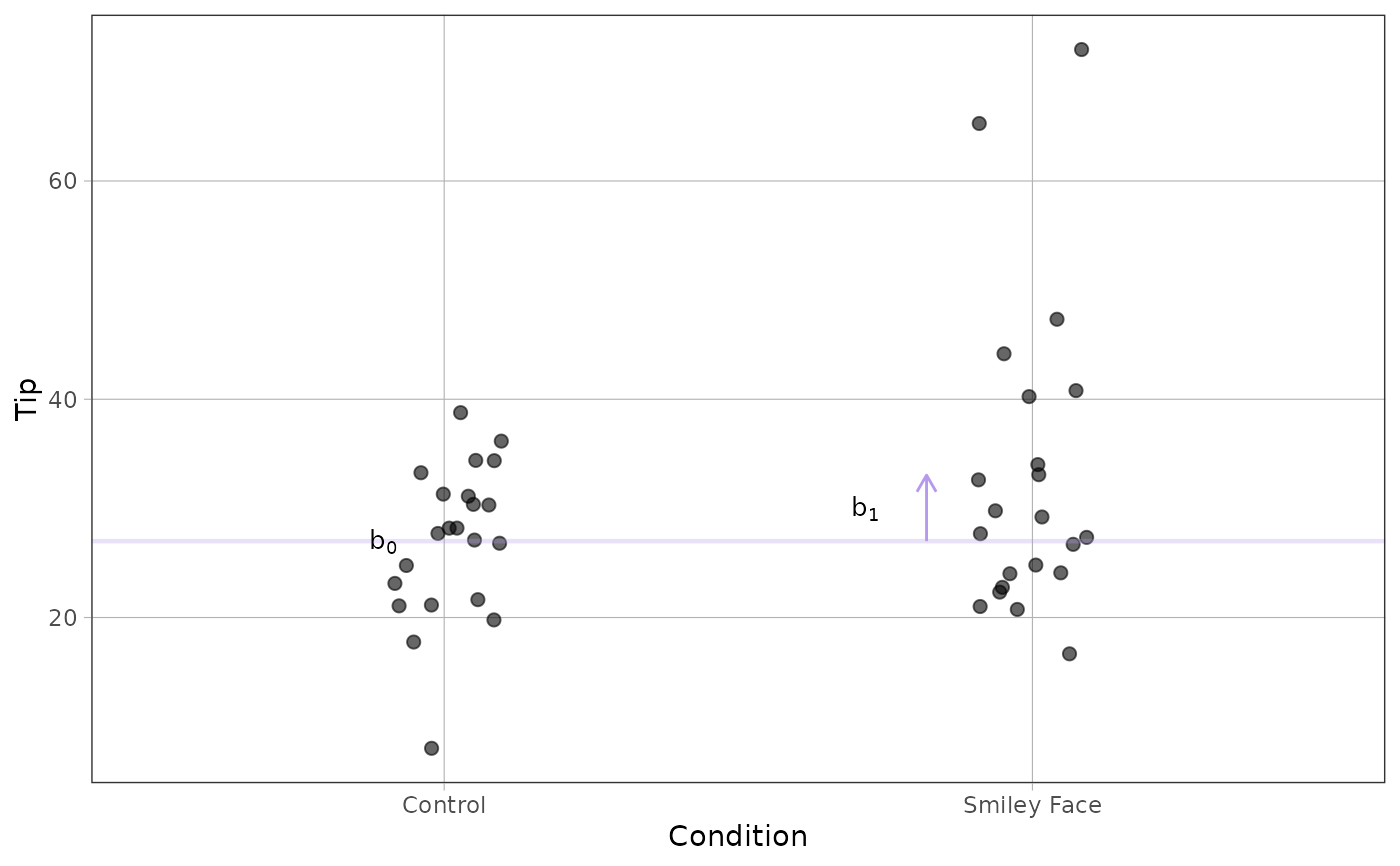
A categorical predictor: one horizontal reference line at b0 (the reference level's mean), and for each level after it a segment from b0 to b0 plus that level's coefficient, with an arrow head, labeled (plotmath) b1, b2, … Level order is read off coef(model), so a releveled factor still labels the arrow that matches its coefficient.

No predictor (the empty model): the b0 line and its label, nothing else.

Every mark is a separately tagged layer – "b0", "b1", "bk_2", "run", and each one's own "_label" – so a script can find one without counting layers.

No model

With no model, gf_b() reads the model the plot implies – the same decision gf_model()'s own inference reads – and fits it at call time, on the plot's whole data. This is refused on a faceted plot, because gf_model()'s inferred line is fit per panel and a single set of arrows drawn over it would describe a fit no panel actually has.

Placement

Every mark is placed from the model's coefficients and from level indices, never from a drawn point's position, so jitter never moves an arrow.

show_b0 = TRUE (the default) expands the PREDICTOR's axis to include 0 on a continuous model, because b0 is the prediction where the predictor is 0 and a picture of it that does not show that point is not a picture of b0. Usually that is x; on a plot that puts the outcome on x it is y, and the expansion follows the predictor rather than the letter. Calling gf_lims() on that axis afterward overrides the expansion and can push the b0 dot off the page.

Examples

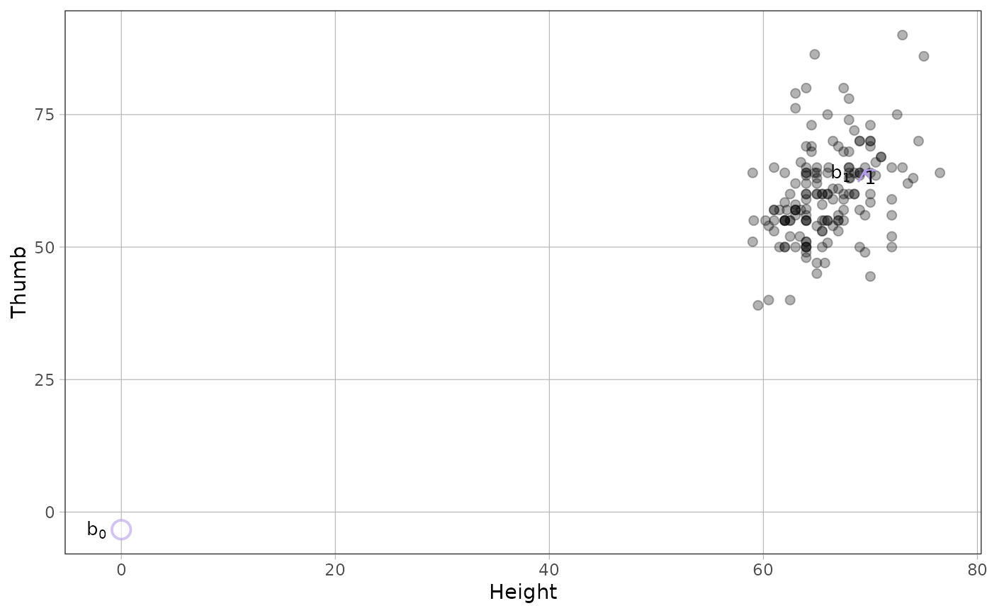
# continuous: b1 as a rise-over-run triangle, b0 where the line meets x = 0
height_model <- lm(Thumb ~ Height, data = Fingers)
gf_point(Thumb ~ Height, data = Fingers, alpha = .3) %>% gf_b(height_model)


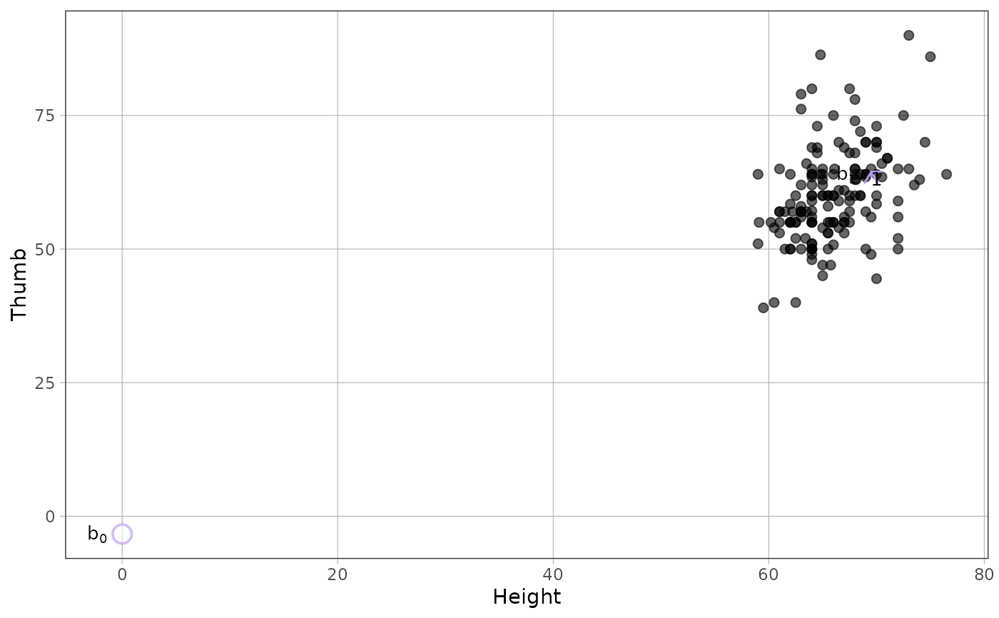
# the slope per one unit
gf_point(Thumb ~ Height, data = Fingers) %>% gf_b(height_model, run = 1)


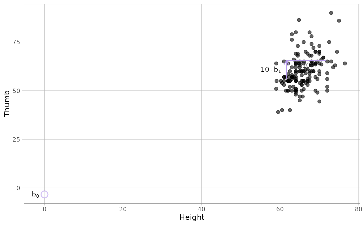
# an explicit run labels the rise "10 x b1"
gf_point(Thumb ~ Height, data = Fingers) %>% gf_b(height_model, run = 10)


# categorical: b0 is the reference group's mean, each b_k is an arrow to group k
tip_model <- lm(Tip ~ Condition, data = TipExperiment)
gf_jitter(Tip ~ Condition, data = TipExperiment, width = .1) %>% gf_b(tip_model)


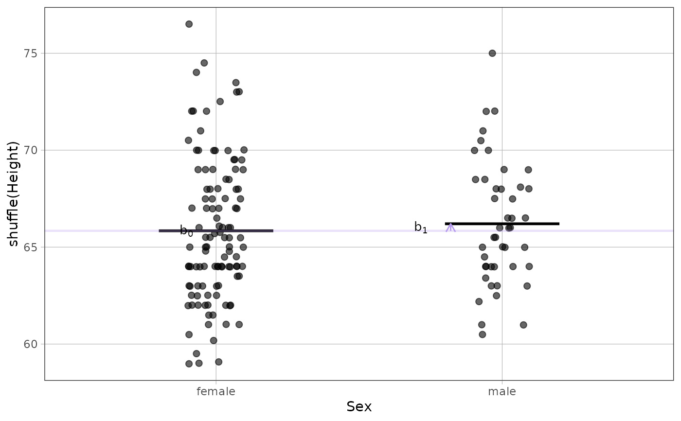
# no model: the model the plot implies, on the values the plot drew
set.seed(1)
gf_jitter(shuffle(Height) ~ Sex, data = Fingers, width = .1) %>%
  gf_model() %>%
  gf_b()


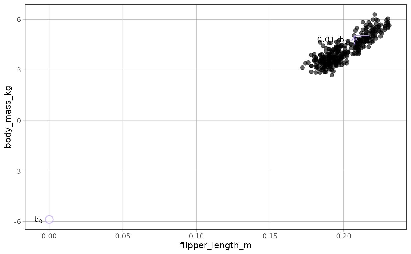
# gf_coef() is the same function under the name coef() readers look for
flipper_model <- lm(body_mass_kg ~ flipper_length_m, data = penguins)
gf_point(body_mass_kg ~ flipper_length_m, data = penguins) %>%
  gf_coef(flipper_model)