Add a Standard Deviation Ruler to a Plot

Usage

gf_sd_ruler(
  object = NULL,
  gformula = NULL,
  data = NULL,
  ...,
  where = "middle",
  na.rm = TRUE,
  xlab,
  ylab,
  title,
  subtitle,
  caption,
  geom = "segment",
  stat = coursekata::StatSdRuler,
  position = "identity",
  show.legend = NA,
  show.help = NULL,
  inherit = TRUE,
  environment = parent.frame()
)

Arguments

object

The plot or data to add the ruler to; typically a plot piped in from gf_point(), gf_jitter(), or gf_histogram().

gformula

A formula naming the outcome and, optionally, the x variable: y ~ x. Defaults to the plot's own mapping when the plot already names one.

data

Dataset. Defaults to the plot's data.

...

Additional arguments: color (default "red"), linewidth (default 0.8), and any other ggplot2::geom_segment() parameter.

where

For a vertical ruler, where on the x-axis to place it: "middle" (midpoint of x range), "mean", or "median". Ignored for a horizontal ruler, which always starts at the mean.

na.rm

Should missing values be silently removed?

xlab, ylab, title, subtitle, caption

Axis and plot labels; see ggformula::gf_point().

geom, stat, position

Layer components; see ggformula::gf_point().

show.legend

Should this layer be included in the legends?

show.help

If TRUE, display some minimal help.

inherit

A logical indicating whether default attributes are inherited from a parent plot.

environment

An environment in which to evaluate the formula.

Value

A ggplot object with the SD ruler segment added.

Details

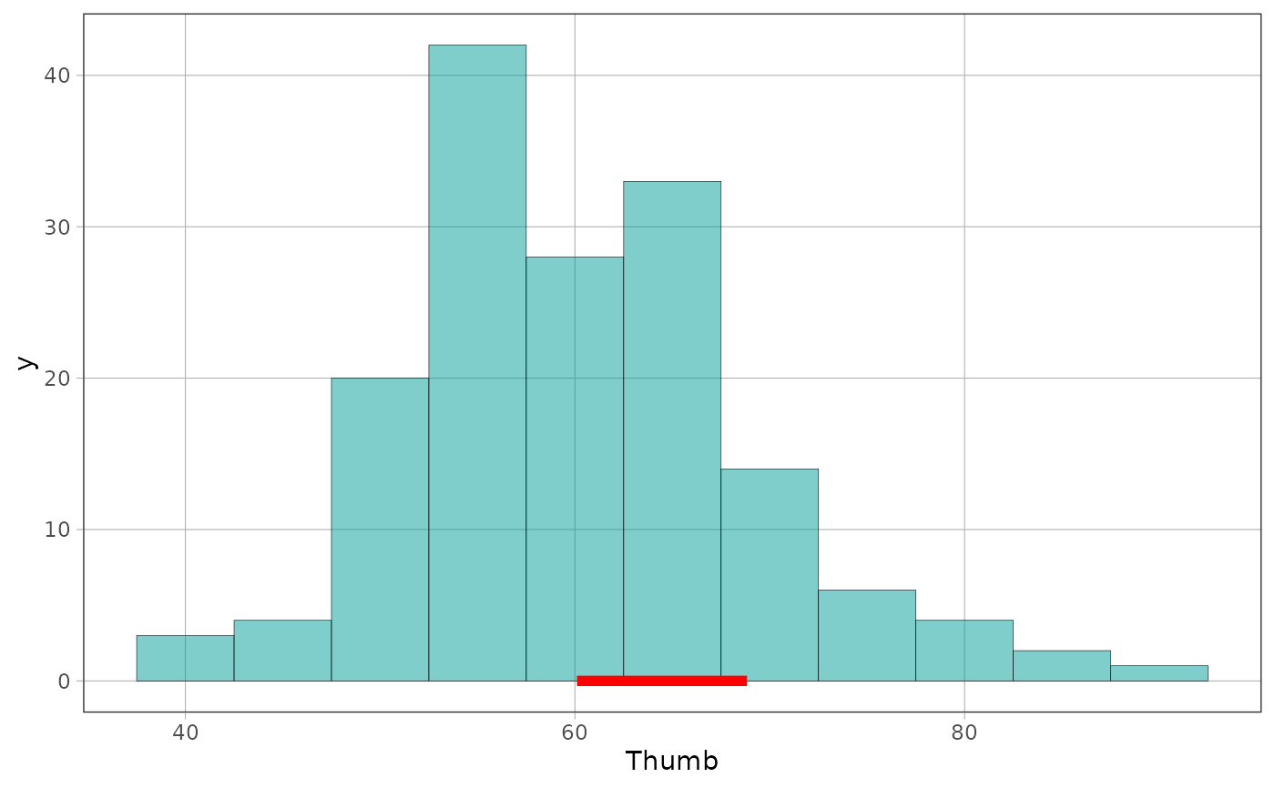
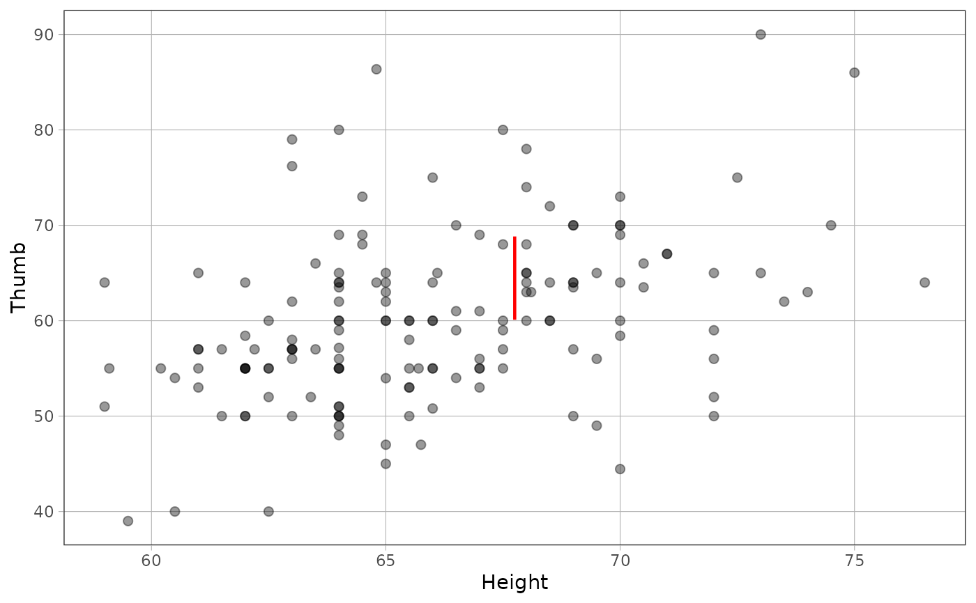
Adds a segment showing one standard deviation of the outcome, anchored at its mean. The orientation depends on where the outcome variable lives: on a scatter or jitter plot (outcome on the y-axis) the ruler is a vertical segment placed at a chosen x position; on a histogram (outcome on the x-axis, no y aesthetic) it is a horizontal segment running from the mean to mean + SD along the baseline. The orientation is detected automatically from the plot's axis mappings.

Both the outcome and, where relevant, the placement are measured in the space the panel is drawn in: a faceted plot measures each panel's own subset, and a transformed axis or a computed mapping such as ~log(Thumb) is measured in the transformed or computed values, not the raw column.

gf_sd_ruler() draws one ruler per panel, so an aesthetic mapped on the call – gf_sd_ruler(color = ~Sex) – is refused; split the plot instead with y ~ x | group to get one ruler per group.

See also

The model visualization guide shows the ruler alongside residuals and compares groups with different spread: https://coursekata.github.io/coursekata-r/articles/model-visualization.html

Examples

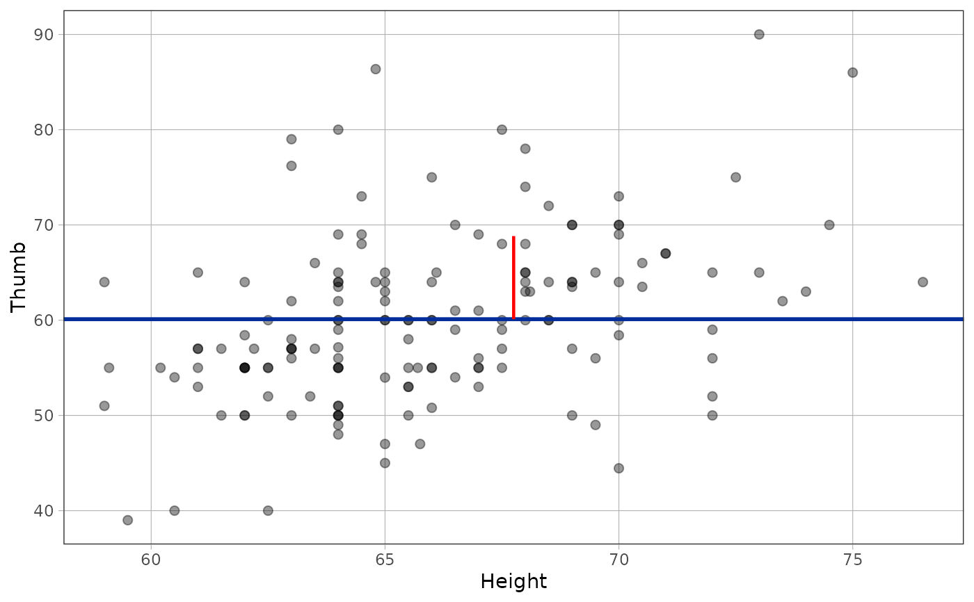
# the ruler runs from the mean (the empty model) up by one standard
# deviation -- it looks like a residual because SD is a typical residual
gf_point(Thumb ~ Height, data = Fingers, alpha = .4) %>%
  gf_model(lm(Thumb ~ NULL, data = Fingers)) %>%
  gf_sd_ruler()


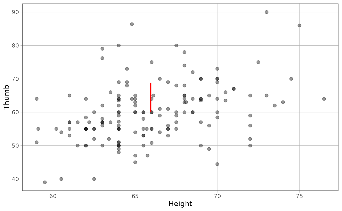
# `where` controls placement along the x-axis
gf_point(Thumb ~ Height, data = Fingers, alpha = .4) %>%
  gf_sd_ruler(where = "mean")


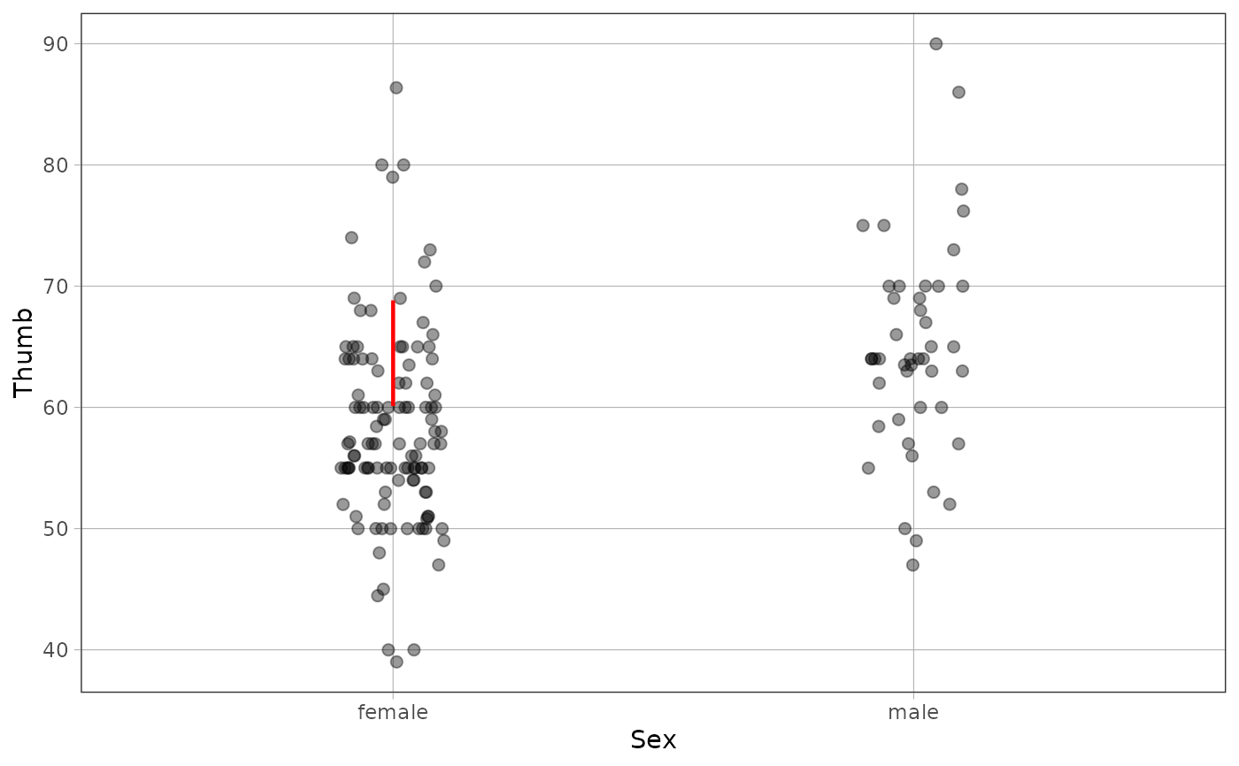
# categorical x works the same way
gf_jitter(Thumb ~ Sex, data = Fingers, width = .1, alpha = .4) %>%
  gf_sd_ruler(where = "median")


# on a histogram the outcome is on the x-axis, so the ruler is horizontal
# and runs along the baseline from the mean to one SD above it
gf_histogram(~Thumb, data = Fingers, binwidth = 5) %>%
  gf_sd_ruler(linewidth = 2)


# name the variable explicitly when the plot does not make it obvious
gf_point(Thumb ~ Height, data = Fingers, alpha = .4) %>%
  gf_sd_ruler(Thumb ~ Height)


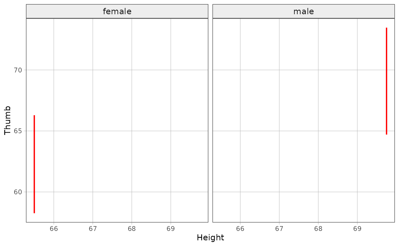
# one ruler per panel
gf_sd_ruler(Thumb ~ Height | Sex, data = Fingers)