
A model’s coefficients are numbers in a table. gf_b()
puts them on the plot, so you can see what each one measures.
In a ggplot2 plot, add geom_b(model = fit) for the same
annotation:
fit <- lm(Thumb ~ Height, data = Fingers)
ggplot2::ggplot(Fingers, ggplot2::aes(Height, Thumb)) +
  ggplot2::geom_point(alpha = .4) + geom_model(model = fit) +
  geom_b(model = fit)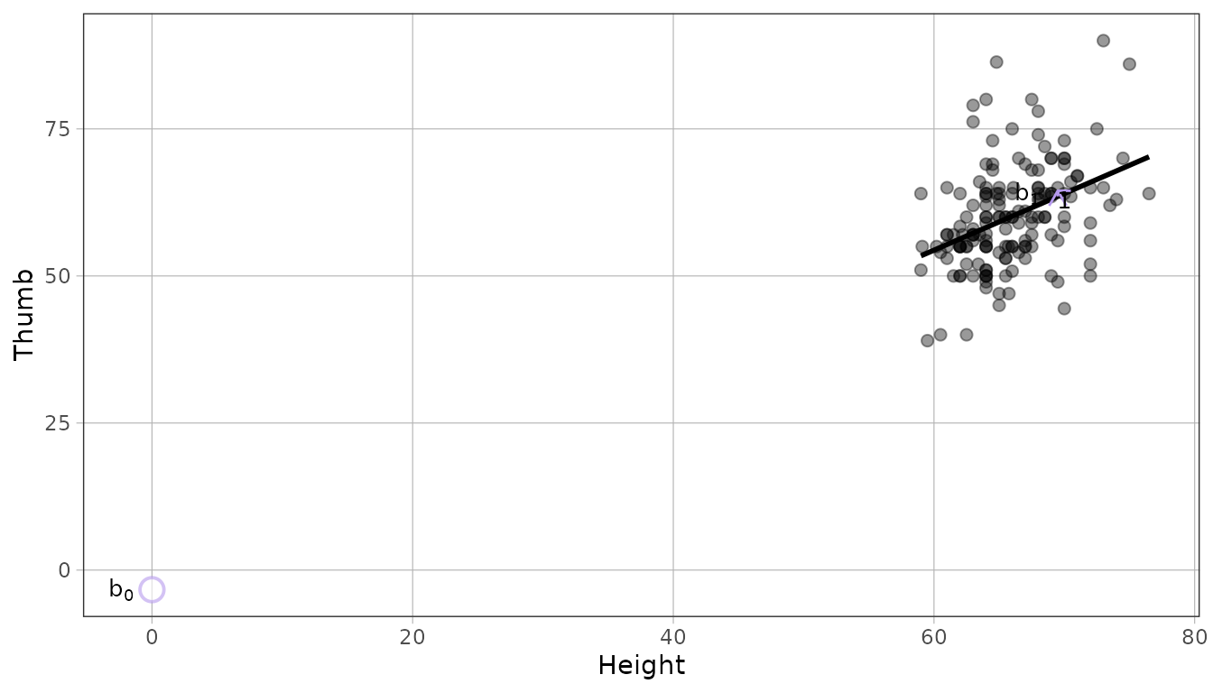
You can omit the model to annotate the plot’s implied fit. The annotation reads the final scales and rows, including limits added later in the pipeline. A supplied fit keeps its original coefficients even when limits hide observations.
gf_point(Thumb ~ Height, data = Fingers) %>%
  gf_lims(x = c(60, 72)) %>%
  gf_model() %>%
  gf_b(show_b0 = FALSE)
#> Warning: Removed 12 rows containing non-finite outside the scale range
#> (`stat_model()`).
#> Warning: Removed 12 rows containing missing values or values outside the scale range
#> (`geom_point()`).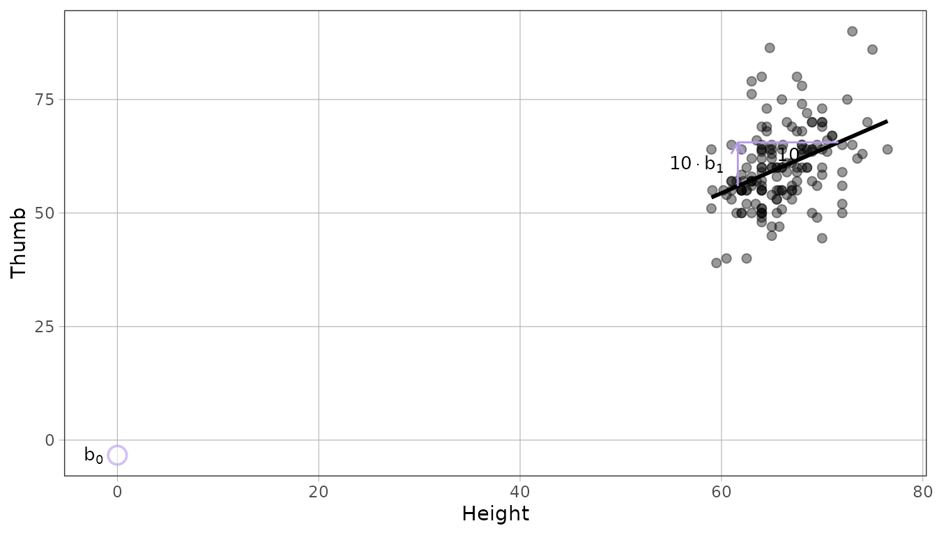
For an inferred model on a transformed scale, the run is measured in
the transformed units. On a log10 predictor scale, run = 1
means a tenfold change in the original predictor. A coordinate zoom
changes the view without changing the rows used to fit the model.
Slope is rise over run
For a quantitative predictor, b1 is how much the
prediction moves for a one-unit change in the predictor.
gf_b() draws that as a triangle.
thumb_model <- lm(Thumb ~ Height, data = Fingers)
gf_point(Thumb ~ Height, data = Fingers, alpha = .4) %>%
  gf_model(thumb_model) %>%
  gf_b(thumb_model)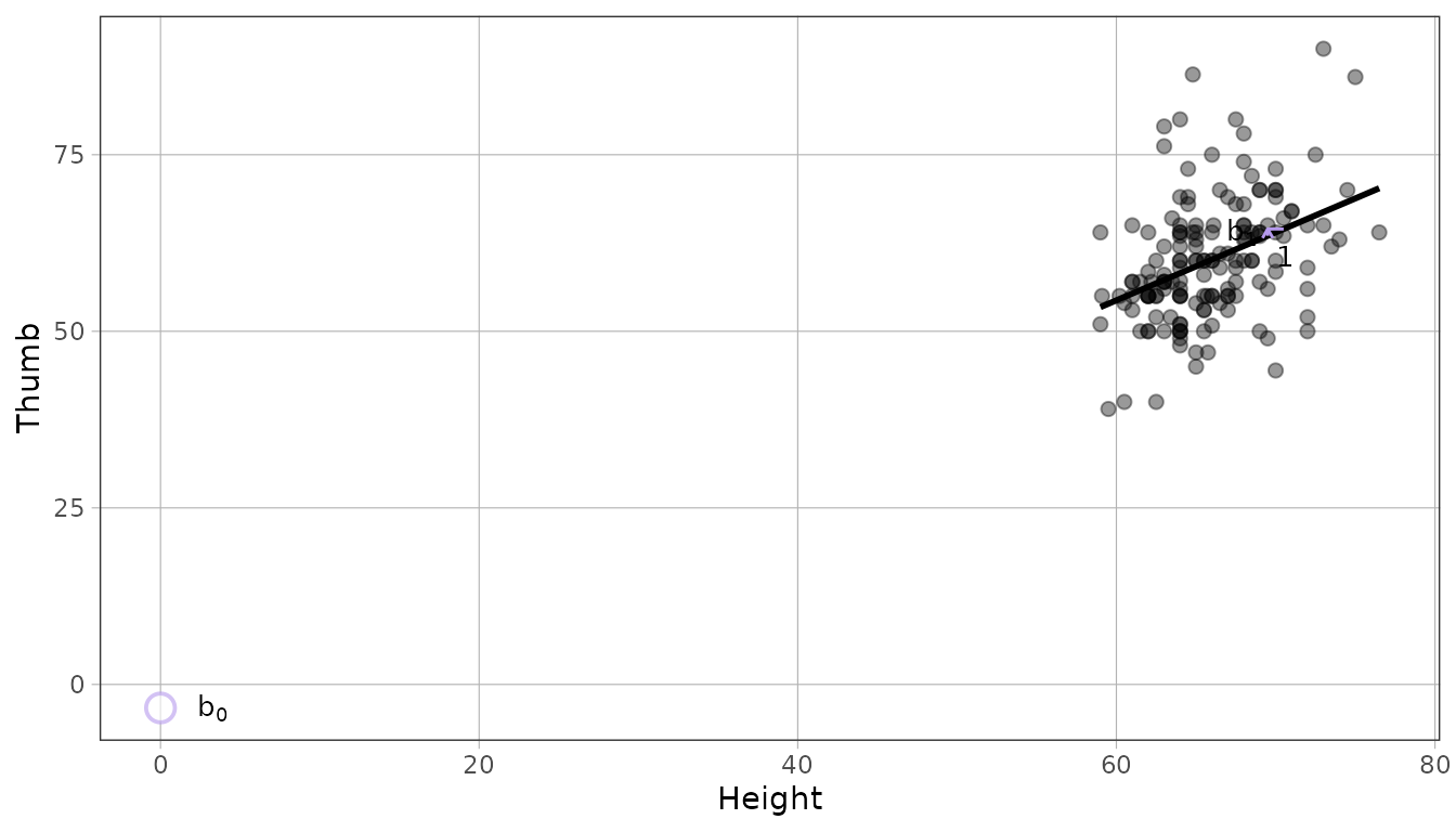
When one unit is too small to see, ask for a longer run. The label says which multiple it is showing.
gf_point(Thumb ~ Height, data = Fingers, alpha = .4) %>%
  gf_model(thumb_model) %>%
  gf_b(thumb_model, run = 10)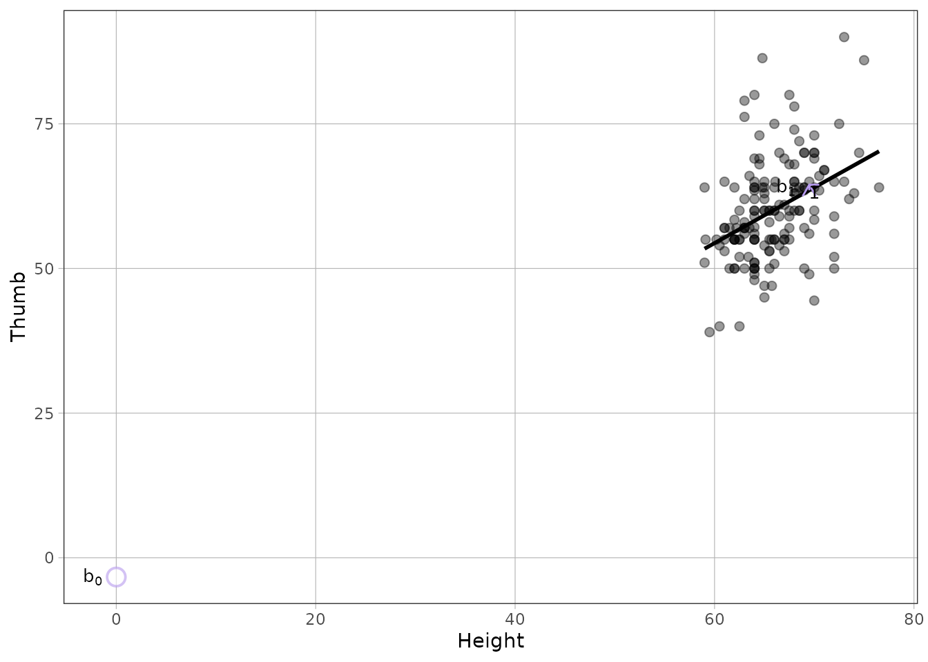
The intercept is a prediction, and it may sit outside the data
b0 is the prediction when the predictor is zero. Here
that is a person of no height, which is why the intercept sits far below
anything the data contains.
coef(thumb_model)
#> (Intercept)      Height
#>  -3.3294866   0.9618834
range(Fingers$Height)
#> [1] 59.0 76.5
The plot makes the distance obvious: to show b0 at all,
the panel has to stretch past every observation.
gf_point(Thumb ~ Height, data = Fingers, alpha = .4) %>%
  gf_model(thumb_model) %>%
  gf_b(thumb_model, show_b0 = TRUE)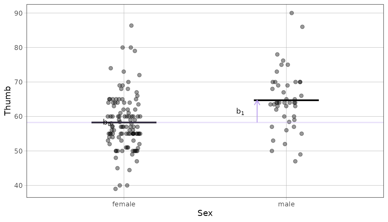
Notice that the line stops well short of the dot. That is deliberate,
and it is worth pausing on. Between the shortest and tallest people in
this sample, every point on the line has observations on both sides of
it. Out at zero there are none, so the line has nothing to stand on and
does not go there. b0 is still a real number the model
reports; the picture is just declining to pretend we watched it
happen.
Centering the predictor moves zero into the data, and b0
becomes the prediction for someone of average height. The slope does not
change.
Fingers$Height_c <- Fingers$Height - mean(Fingers$Height)
centered_model <- lm(Thumb ~ Height_c, data = Fingers)

gf_point(Thumb ~ Height_c, data = Fingers, alpha = .4) %>%
  gf_model(centered_model) %>%
  gf_b(centered_model, show_b0 = TRUE)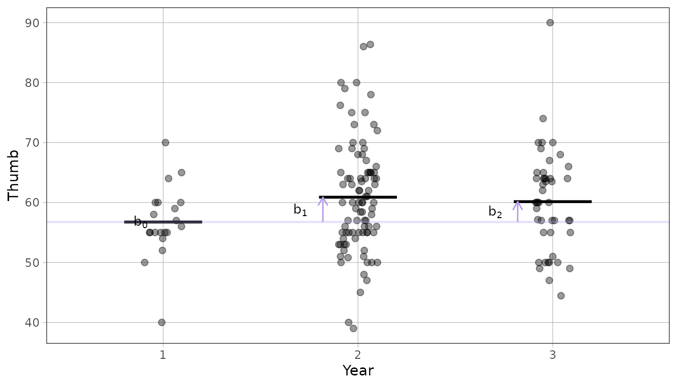
With groups, the coefficients are differences
For a categorical predictor, b0 is the first group’s
mean and each other coefficient is a distance from it. The arrows
measure those distances.
sex_model <- lm(Thumb ~ Sex, data = Fingers)
gf_jitter(Thumb ~ Sex, data = Fingers, width = .1, alpha = .4) %>%
  gf_model(sex_model) %>%
  gf_b(sex_model)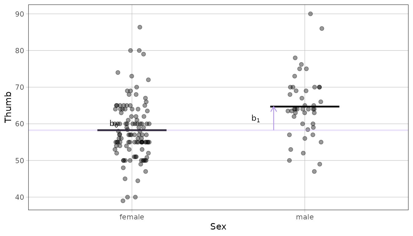
With three groups there are two arrows, both measured from the same reference.
three <- droplevels(subset(Fingers, Year %in% c("1", "2", "3")))
year_model <- lm(Thumb ~ Year, data = three)
gf_jitter(Thumb ~ Year, data = three, width = .1, alpha = .4) %>%
  gf_model(year_model) %>%
  gf_b(year_model)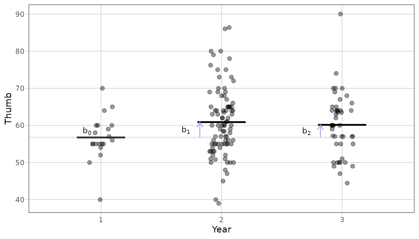
The arrows start where the reference group’s prediction is, so a coefficient that reads as a small number is a short arrow, whatever the outcome’s scale.